

Are you ready to elevate your Excel skills? In this blog, we’re diving into advanced Excel conditional formatting tricks using dynamic formulas and functions. These Excel tips and tricks will help you make your spreadsheets not just functional but also visually appealing and dynamically responsive to changes in your data. Whether you’re a novice or a seasoned Excel user, you’re bound to learn something new.
Conditional Formatting Basics
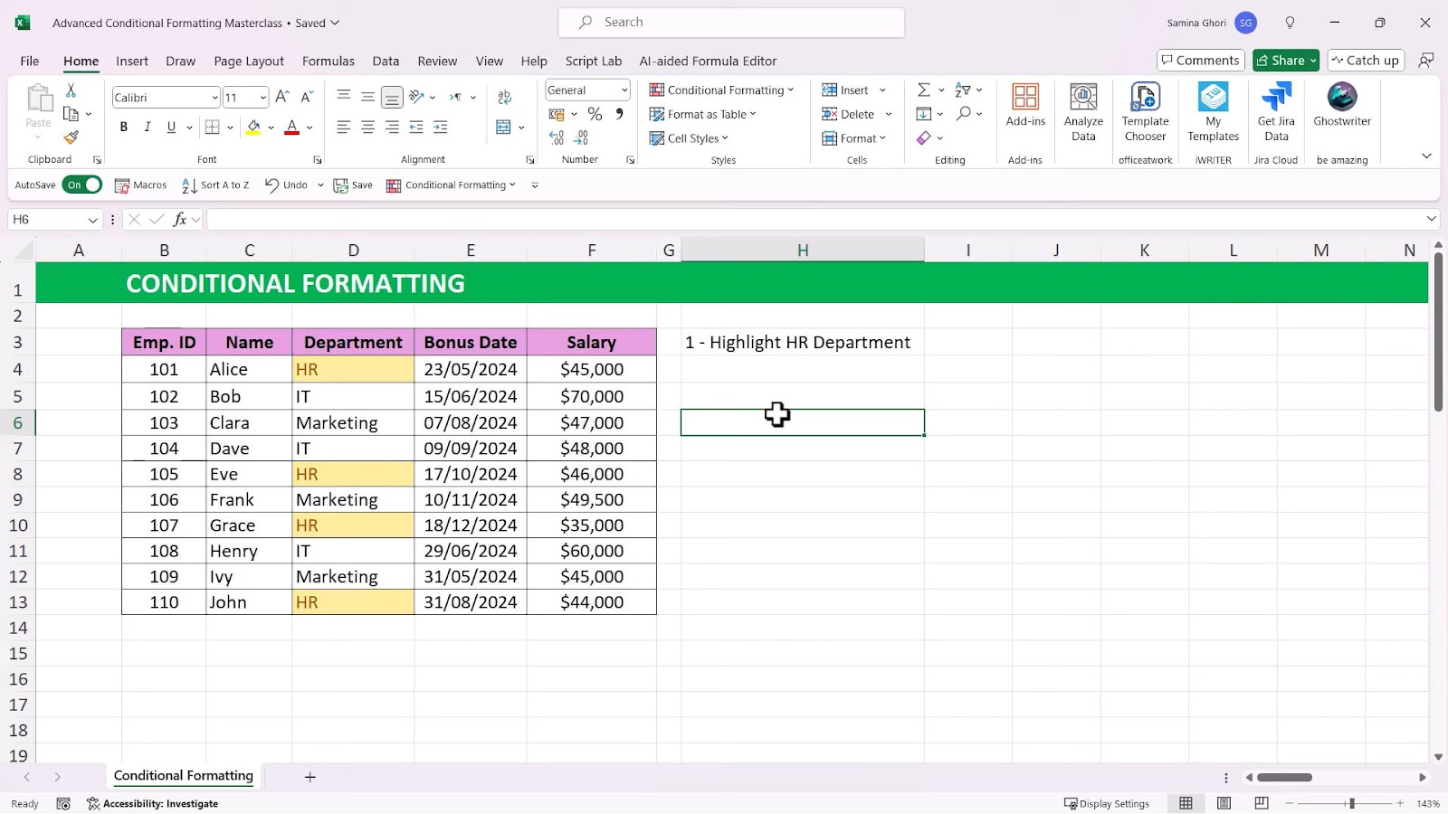
Conditional formatting in Excel allows you to apply specific formatting to cells that meet certain criteria. For example, you might highlight cells that contain specific text or exceed a particular value. This feature is powerful, but many users only scratch the surface of its capabilities.
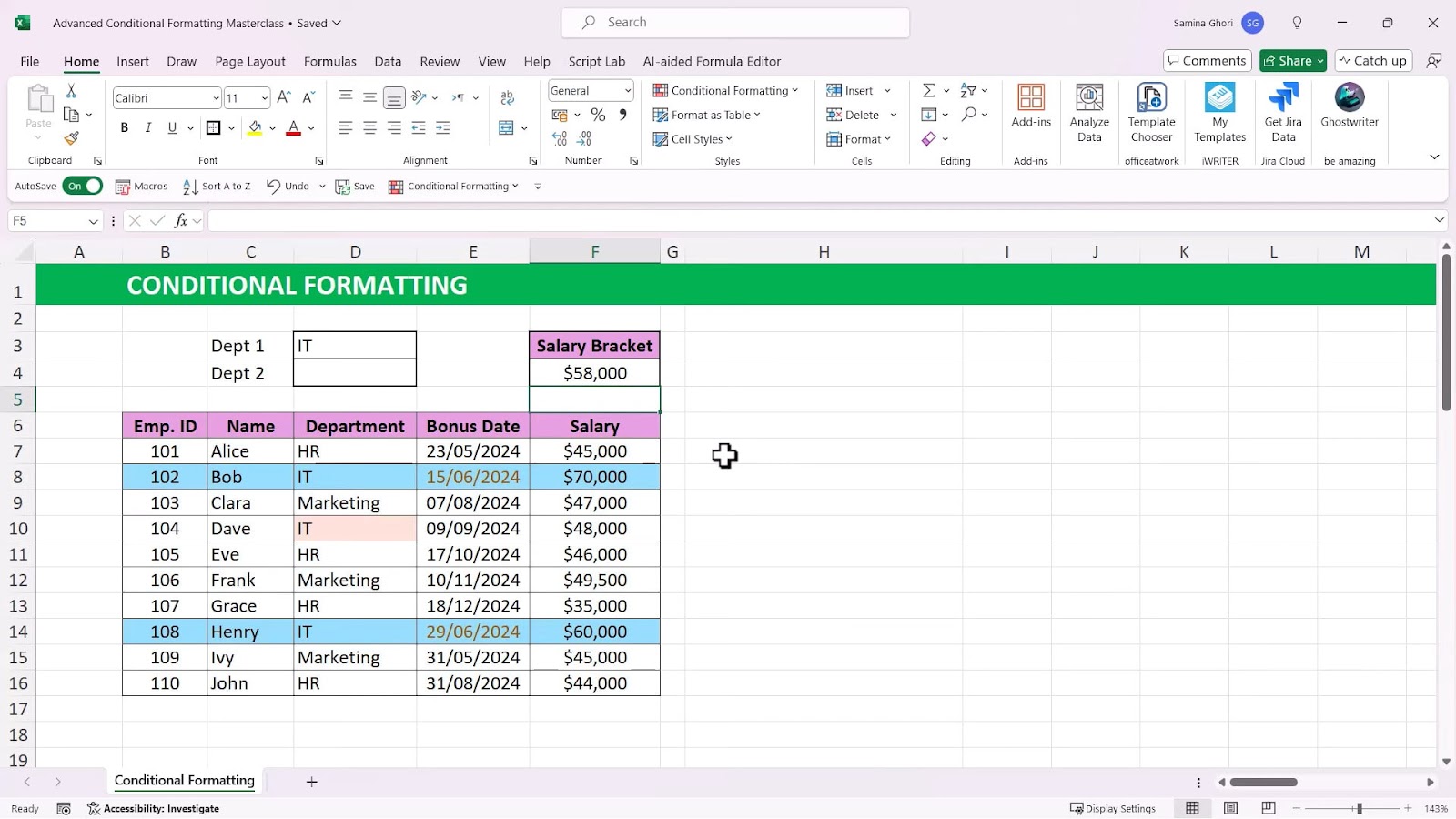
In my video, I begin opposed to I begins with a basic example: highlighting the “HR” department in a spreadsheet. You select your range, go to conditional formatting, and choose “Text that Contains.” But what if you want to highlight multiple departments like “HR” and “IT”? Instead of creating separate rules for each, you can use a dynamic formula.
Using Formulas for Dynamic Text Highlighting
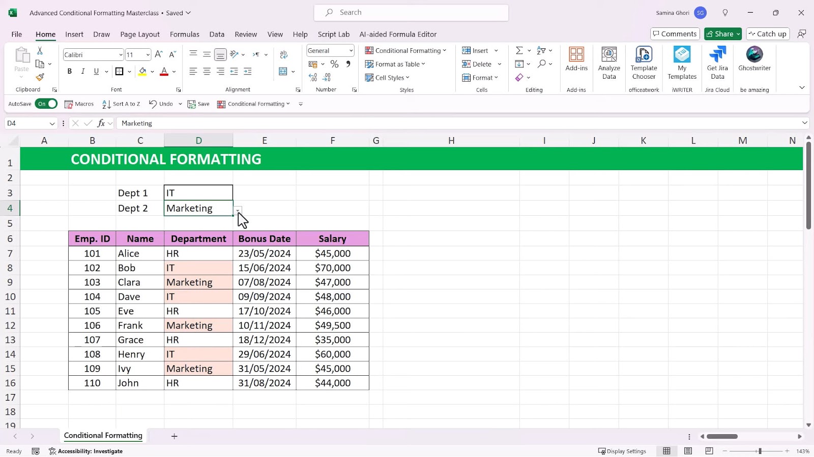
To highlight both “HR” and “IT” departments dynamically, you use a formula. Select your range, go to conditional formatting, and choose to create a new rule using a formula. The formula is simple: =OR(D3=”HR”, D3=”IT”). This way, you can format both departments with a single rule. I demonstrate this by applying an orange colour to the highlighted cells.
For an even more dynamic approach, you can use a data validation list to make the department selection dynamic. This way, the conditional formatting will update based on the selected department from the list, ensuring your formatting rules are always up-to-date.
Highlighting Dates Dynamically
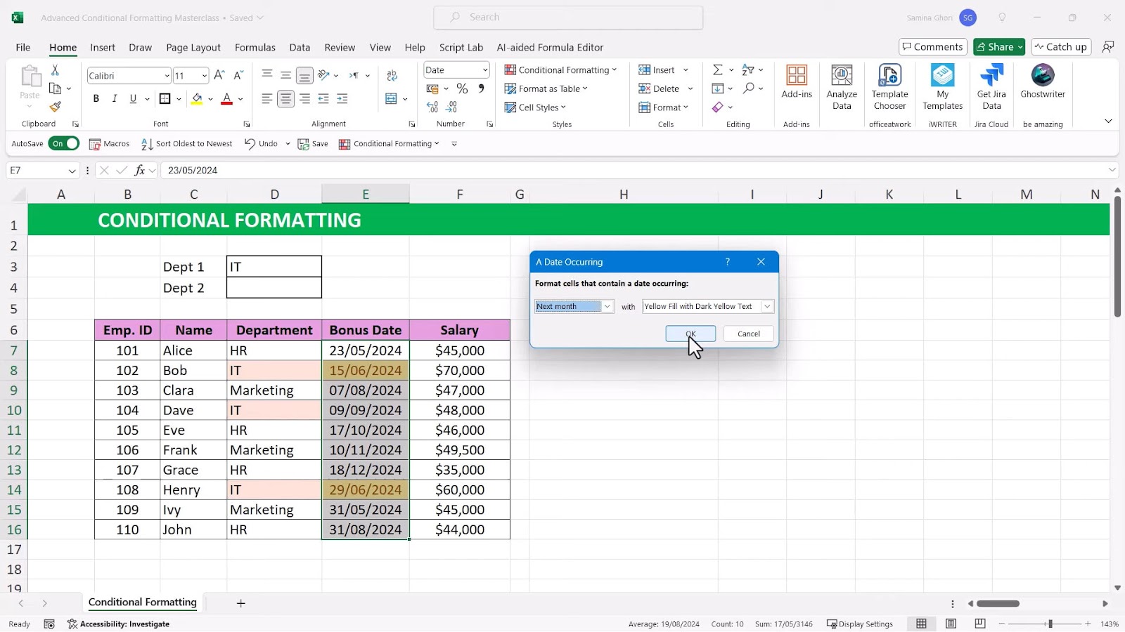
Next, I move on to dates, showing how to highlight cells based on dates relative to the current date. This can be useful for tracking deadlines, birthdays, or any time-sensitive information. You can set rules to highlight cells for dates such as yesterday, today, tomorrow, or within the last seven days. This dynamic approach means you don’t have to manually update your rules – Excel does it for you.
Dynamic Number Range Formatting
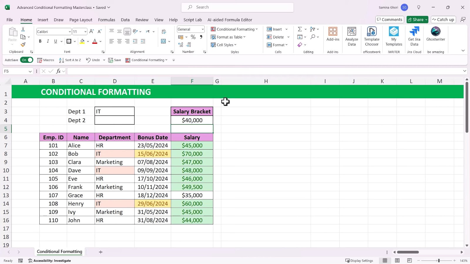
Highlighting cells based on numerical values is another common task. For instance, you might want to highlight salaries above a certain threshold. I show how to do this both statically and dynamically. Instead of hardcoding the value (e.g., $50,000), you can reference a cell. This way, if you change the reference cell value, all relevant cells update automatically. For example, if you want to highlight all salaries above $40,000, you can reference a cell where you input this threshold. This makes your spreadsheet more flexible and easier to maintain.
Row Highlighting Based on Cell Value
Sometimes, you need to highlight entire rows based on a cell’s value. For example, you might want to highlight all rows where the salary exceeds $50,000. I demonstrate this by creating a new rule that uses a formula to determine which cells to format. The key here is to lock the column reference but not the row reference, allowing the formatting to apply to the entire row dynamically.
Visual Data Representation with Colour Scales and Icon Sets
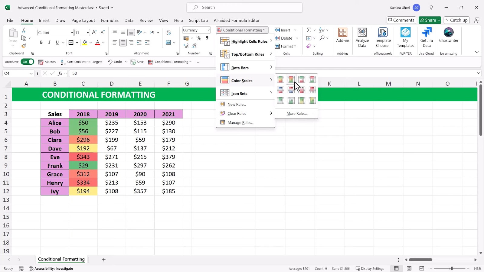
Visual representation of data can make analysis much easier. I cover the use of colour scales and icon sets to give immediate visual feedback on data ranges. Colour scales apply a gradient to your data, with colours representing different values. For example, you might use a green-to-red scale to show high and low values. Icon sets add icons to cells based on their values, such as arrows or traffic lights. You can customize these to fit your specific needs.
Adding Data Bars and Sparklines
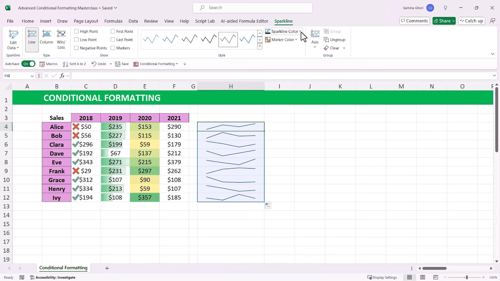
Data bars add horizontal bars to your cells, visually representing the value within the cell. This can be particularly useful for comparing values within a range. I show how to add data bars and customize their appearance.
Sparklines, on the other hand, are tiny charts within a cell that give a quick visual representation of data trends over time. You can use them to show trends for sales data, for instance. I explain how to create both line and column sparklines, highlighting high and low points within your data.
Highlighting Weekends Using the WEEKDAY Function
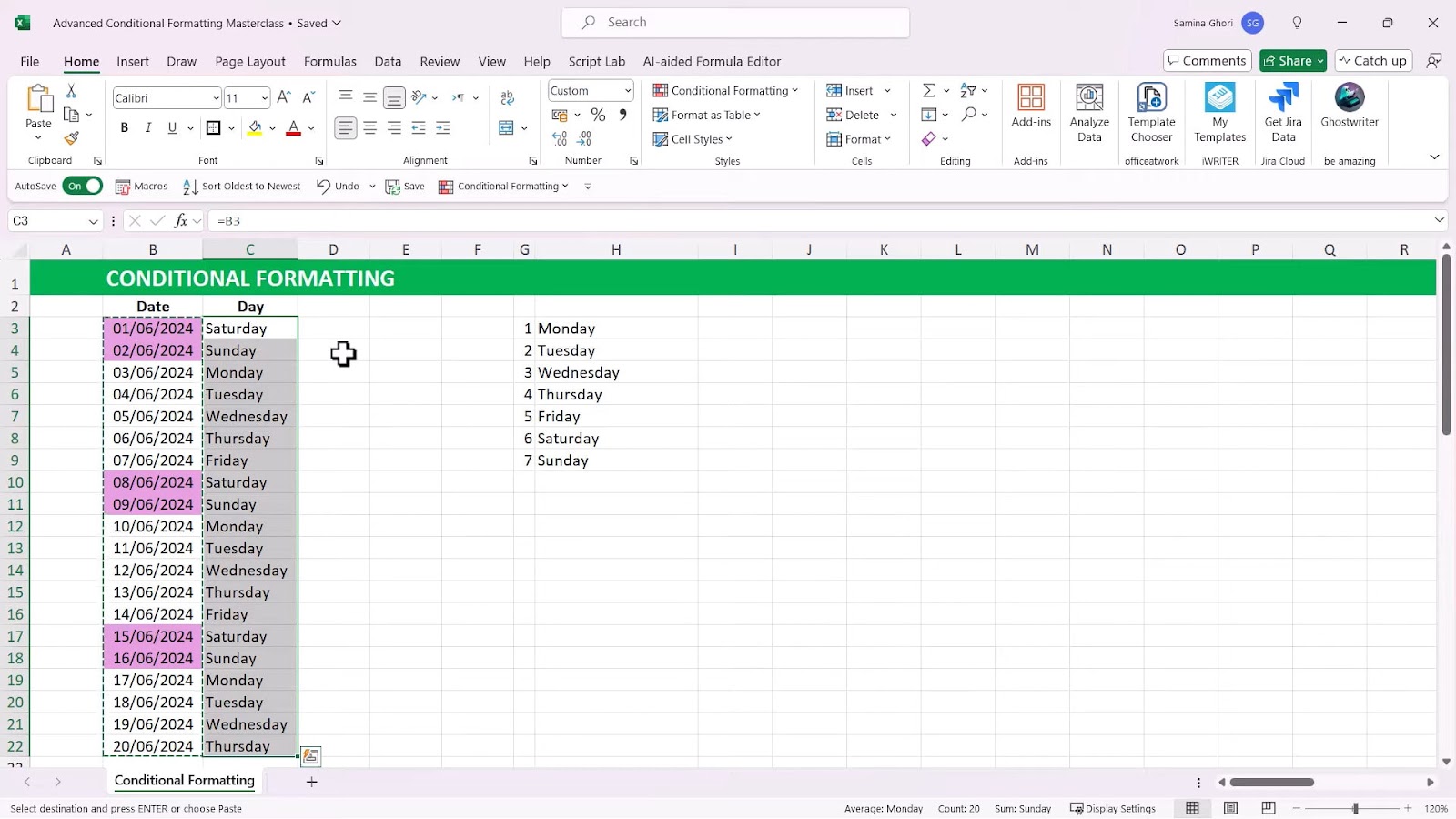
Highlighting weekends can be tricky since Excel doesn’t recognize days as text. Instead, you use the WEEKDAY function, which assigns numbers to days (e.g., Monday is 1, Sunday is 7). I demonstrate how to create a conditional formatting rule that highlights weekends using this function. By applying a formula =WEEKDAY(A2,2)>5, you can dynamically highlight Saturdays and Sundays.
Conclusion
Advanced Excel conditional formatting is a game-changer for anyone looking to make their data more visually appealing and easier to interpret. By using dynamic formulas and functions, you can create flexible, responsive formatting rules that save time and reduce errors. Whether you’re tracking deadlines, comparing sales data, or highlighting key information, these techniques will help you get the most out of Excel.
Why You Should Watch This Video
If you found these tips useful, be sure to watch the full video of mine on my channel Samina Ghori on “Advanced Excel Conditional Formatting Tricks using Dynamic Formulas & Functions” to see these techniques in action. I walk through each step with clear examples, helping you master conditional formatting and become an Excel pro. Click here to watch the video now!
FAQs
1. What is conditional formatting in Excel?
Conditional formatting is a feature in Excel that allows you to apply specific formatting to cells that meet certain criteria.
2. How do I highlight cells based on text content?
You can use the “Text that Contains” rule in conditional formatting, or for multiple texts, use a formula like =OR(D3=”HR”, D3=”IT”).
3. Can I highlight cells based on dynamic date ranges?
Yes, you can set rules to highlight cells based on dates relative to the current date, such as yesterday, today, or within the last seven days.
4. How do I use data bars and sparklines?
Data bars visually represent values within cells using horizontal bars. Sparklines are tiny charts within cells that show trends over time. Both can be added via the Insert menu.
5. How can I highlight weekends in my Excel sheet?
You can use the WEEKDAY function in a conditional formatting formula to highlight weekends dynamically.